What an Audio Interface Can Capture Across the VLF Band
How can an independent researcher capture military submarine communications and ionospheric heating sidebands using off-the-shelf audio hardware?
Start with the receiver’s actual bandwidth. A USB audio interface with a verified analog response across 3–30 kHz can sample very low frequency signals directly at 96 or 192 kHz, without a radio-frequency downconverter. The accurate description is direct sampling. Only the lower portion of VLF overlaps ordinary human hearing.
That makes a modest listening station possible. It also puts the first purchasing decision somewhere easily overlooked: the interface’s frequency-response specification. A high sample-rate setting alone says little about what reaches the converter. Some audio inputs attenuate signals above approximately 20 kHz; check the specification and verify reception at 24–30 kHz before committing to the hardware.
The build has three essential parts:
- A multi-turn magnetic loop with electrostatic shielding to reduce local electric-field pickup.
- A balanced, low-noise input chain, with differential amplification where needed and a suitable transformer when galvanic isolation is required.
- A high-sample-rate USB audio interface feeding raw recordings and spectrum-analysis software.
A transformer provides isolation; amplification requires a powered stage. Keep those jobs separate when comparing components. The Stanford VLF Group receiver documentation provides further receiver background.
For investigations touching intelligence and conflicts, the useful starting point is a reproducible electromagnetic measurement, with interpretation attached afterward.
Build the Loop Around Its Measured Response
A one-meter-square frame gives each turn approximately one square meter of enclosed area. Wind 50–100 turns around that perimeter and the project consumes approximately 200–400 meters of conductor before feedline and termination allowances. This is a substantial winding, so rigidity matters.
Use schedule 40 PVC or dry wooden supports. A square frame or supported octagonal arrangement should hold the wire without changing shape during a recording. Secure the winding as you go, and record the actual enclosed area.
Use 22–24 AWG enameled copper wire, treating the proposed turn count as a prototype. More turns increase induced voltage, while added inductance and distributed capacitance can bring resonance into the receiving band. Measure the completed winding’s impedance or swept response through 3–30 kHz before fixing the final arrangement.
Keep the Shield Electrically Open
Wrap the coil bundle in conductive copper or aluminum foil tape, leaving a roughly 10-millimeter insulating break at the top. That break must pass through every conductive layer. Overlapping foil, conductive adhesive, or a drain wire bridging it can recreate a closed turn and weaken magnetic reception.
Connect the shield to one designated receiver-side shield or chassis reference. Keep that connection distinct from the balanced input’s cold terminal, which carries signal.
The broader principle is simple: the winding geometry and shield construction belong in the measurement record. A recording made after moving the turns or bridging the shield gap comes from a changed antenna.
Protect the Input Without Losing the Upper VLF Band
Assemble and test the receiver indoors first. Route the loop’s twisted-pair feedline into a balanced, low-noise chain. Where isolation is needed, select a 1:1 transformer with documented response through 30 kHz, then use a suitable differential preamplifier or balanced interface input.
An ordinary audio transformer may roll off in the very band being investigated. Likewise, a preamplifier’s line-level output belongs on a line input. Keep phantom power disabled unless every connected component explicitly accepts it.
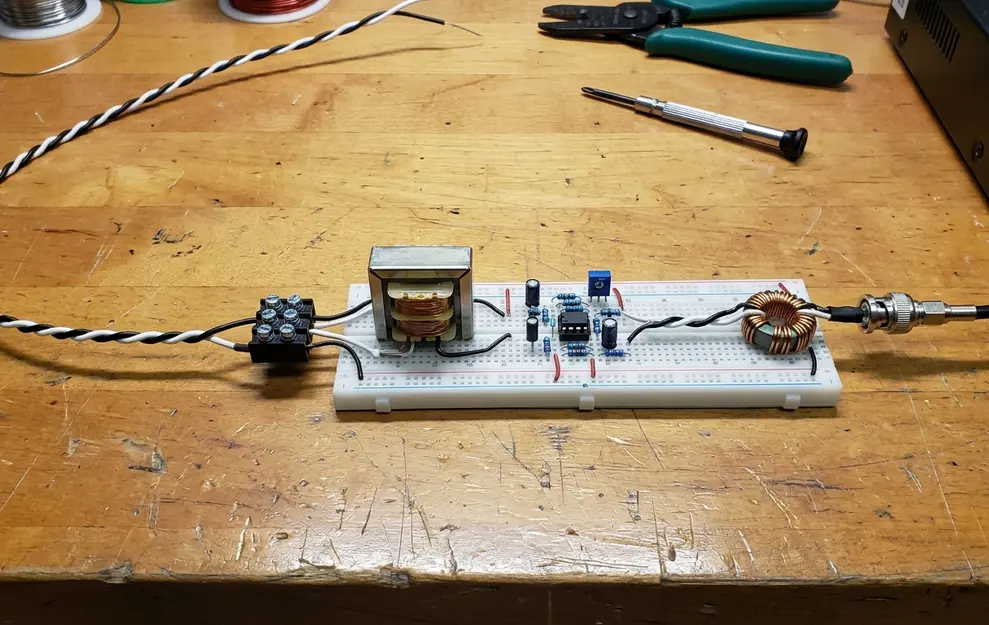
Set the interface to its native 96 or 192 kHz rate and record uncompressed PCM. Disable automatic gain control, noise suppression, echo cancellation, equalization, and operating-system audio enhancements.
Watch the complete input spectrum while setting gain. Strong 50/60 Hz pickup and its harmonics can overload the analog stage before the desired carrier looks large on screen. Reduce gain or remove the interference source whenever the waveform clips.
Disconnect Before Storms
An isolation transformer can interrupt a conductive ground-loop path. It provides no lightning protection. Disconnect portable equipment and bring it indoors before thunderstorms; keep the loop away from mains wiring and utility grounds.
Check the shield wiring too. An extra connection across the transformer’s isolation barrier can defeat the separation the transformer supplies.
Choose FFT Settings That Deliver the Claimed Resolution
How narrow are the frequency bins actually displayed on the waterfall?
I start with that calculation before interpreting a thin trace. Use vlfrx-tools for an open-source VLF processing option. Spectrum Lab is another established analysis application. Feed the software the raw PCM stream and verify the frequency scale against a suitable reference.
FFT bin spacing equals sample rate divided by transform length. At 96 kHz, a 65,536-point FFT produces approximately 1.46 Hz bins. At 192 kHz, the same transform produces approximately 2.93 Hz bins.
For approximately 0.732 Hz spacing, select 131,072 points at 96 kHz or 262,144 points at 192 kHz. Each transform spans approximately 1.365 seconds. A Hann window reduces leakage while broadening the effective response, so retain the window and averaging settings with the recording.
Repeat the Directional Null
With a persistent transmitter visible, rotate the vertically mounted loop through a complete turn. Look for two opposing minima, then repeat the rotation. Log orientation, gain, and frequency at each repeatable minimum.
A reproducible null supports directional magnetic reception. Local magnetic interference can also have directionality. Preserve comparison recordings while switching nearby chargers, lighting drivers, and computers off individually. That comparison helps separate antenna behavior from the room’s electrical activity.
Run a Sunset Session Around the 24 kHz NAA Signal
Set the completed receiver away from residential power lines and use NAA at Cutler, Maine, commonly listed at 24.0 kHz, as the candidate signal. Confirm current station information and on-air presence before starting. Treat the following sequence as an observation plan.
Receiving a naval transmission establishes reception, rather than access to its message or evidence that neighboring traces originate from an ionospheric heater.
- Open the record before sunset. Begin 20 minutes before local sunset and continue until 40 minutes afterward. Record the location, sunset calculation, and clock-synchronization status. Twilight propagation follows the complete transmitter–receiver path.
- Locate the candidate transmission. Center the display near 24.0 kHz. Expect MSK energy across a band around the nominal center frequency. Use frequency and independently checked station information for identification; an ordinary waterfall does not directly display individual phase transitions.
- Fix the gain and preserve the waveform. Save lossless PCM WAV audio with the UTC start time in the filename. Keep a companion log containing sample rate, bit depth, channel count, gain, loop orientation, FFT settings, and any missing samples. Record amplitude in relative units or dBFS.
- Examine changes against competing explanations. For a sudden amplitude drop, check clipping indicators and local switching activity, then compare the interval with NOAA Space Weather Prediction Center solar X-ray observations. Examine 3–10 kHz separately. Any heater attribution requires independently documented operating times, compatible modulation, and corroborating observations.
- Close the session with an auditable event entry. Select an amplitude change in the saved recording, enter its UTC time, retain the surrounding waveform, and pair it with the gain and orientation log. Add the corresponding local-switching notes and solar X-ray comparison. If investigating heating, attach available operating logs and geomagnetic indices for that same interval. The resulting entry ties one observed change to the exact receiver state and comparison records needed to examine it.